Convolution in the context of Complex frequency


Convolution in the context of Complex frequency

Convolution Study page number 1 of 1

Play TriviaQuestions Online!

or

Skip to study material about Convolution in the context of "Complex frequency"


⭐ Core Definition: Convolution

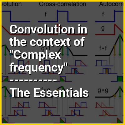
In mathematics (in particular, functional analysis), convolution is a mathematical operation on two functions and that produces a third function , as the integral of the product of the two functions after one is reflected about the y-axis and shifted. The term convolution refers to both the resulting function and to the process of computing it. The integral is evaluated for all values of shift, producing the convolution function. The choice of which function is reflected and shifted before the integral does not change the integral result (see commutativity). Graphically, it expresses how the 'shape' of one function is modified by the other.

Some features of convolution are similar to cross-correlation: for real-valued functions, of a continuous or discrete variable, convolution differs from cross-correlation only in that either or is reflected about the y-axis in convolution; thus it is a cross-correlation of and , or and . For complex-valued functions, the cross-correlation operator is the adjoint of the convolution operator.

↓ Menu
HINT:

In this Dossier

Convolution in the context of Time averaging

In statistics, a moving average (rolling average or running average or moving mean or rolling mean) is a calculation to analyze data points by creating a series of averages of different selections of the full data set. Variations include: simple, cumulative, or weighted forms.

Mathematically, a moving average is a type of convolution. Thus in signal processing it is viewed as a low-pass finite impulse response filter. Because the boxcar function outlines its filter coefficients, it is called a boxcar filter. It is sometimes followed by downsampling.

View the full Wikipedia page for Time averaging
↑ Return to Menu

Convolution in the context of Laplace transform

In mathematics, the Laplace transform, named after Pierre-Simon Laplace (/ləˈplɑːs/), is an integral transform that converts a function of a real variable (usually , in the time domain) to a function of a complex variable (in the complex-valued frequency domain, also known as s-domain or s-plane). The functions are often denoted by for the time-domain representation and for the frequency-domain.

The transform is useful for converting differentiation and integration in the time domain into much easier multiplication and division in the Laplace domain (analogous to how logarithms are useful for simplifying multiplication and division into addition and subtraction). This gives the transform many applications in science and engineering, mostly as a tool for solving linear differential equations and dynamical systems by simplifying ordinary differential equations and integral equations into algebraic polynomial equations, and by simplifying convolution into multiplication.

View the full Wikipedia page for Laplace transform
↑ Return to Menu

Convolution in the context of Frequency response

In signal processing and electronics, the frequency response of a system is the quantitative measure of the magnitude and phase of the output as a function of input frequency. The frequency response is widely used in the design and analysis of systems, such as audio equipment and control systems, where they simplify mathematical analysis by converting governing differential equations into algebraic equations. In an audio system, it may be used to minimize audible distortion by designing components (such as microphones, amplifiers and loudspeakers) so that the overall response is as flat (uniform) as possible across the system's bandwidth. In control systems, such as a vehicle's cruise control, it may be used to assess system stability, often through the use of Bode plots. Systems with a specific frequency response can be designed using analog and digital filters.

The frequency response characterizes systems in the frequency domain, just as the impulse response characterizes systems in the time domain. In linear systems (or as an approximation to a real system neglecting second order non-linear properties), either response completely describes the system and thus there is a one-to-one correspondence: the frequency response is the Fourier transform of the impulse response. The frequency response allows simpler analysis of cascaded systems such as multistage amplifiers, as the response of the overall system can be found through multiplication of the individual stages' frequency responses (as opposed to convolution of the impulse response in the time domain). The frequency response is closely related to the transfer function in linear systems, which is the Laplace transform of the impulse response. They are equivalent when the real part of the transfer function's complex variable is zero.

View the full Wikipedia page for Frequency response
↑ Return to Menu

Convolution in the context of Newtonian potential

In mathematics, the Newtonian potential, or Newton potential, is an operator in vector calculus that acts as the inverse to the negative Laplacian on functions that are smooth and decay rapidly enough at infinity. As such, it is a fundamental object of study in potential theory. In its general nature, it is a singular integral operator, defined by convolution with a function having a mathematical singularity at the origin, the Newtonian kernel which is the fundamental solution of the Laplace equation. It is named for Isaac Newton, who first discovered it and proved that it was a harmonic function in the special case of three variables, where it served as the fundamental gravitational potential in Newton's law of universal gravitation. In modern potential theory, the Newtonian potential is instead thought of as an electrostatic potential.

The Newtonian potential of a compactly supported integrable function is defined as the convolution

View the full Wikipedia page for Newtonian potential
↑ Return to Menu

Convolution in the context of Discrete Fourier transform

In mathematics, the discrete Fourier transform (DFT) is a discrete version of the Fourier transform that converts a finite sequence of equally-spaced samples of a function into a same-length sequence of equally-spaced samples of the discrete-time Fourier transform (DTFT), which is a complex-valued function of frequency. The interval at which the DTFT is sampled is the reciprocal of the duration of the input sequence. An inverse DFT (IDFT) is a Fourier series, using the DTFT samples as coefficients of complex sinusoids at the corresponding DTFT frequencies. It has the same sample-values as the original input sequence. The DFT is therefore said to be a frequency domain representation of the original input sequence. If the original sequence spans all the non-zero values of a function, its DTFT is continuous (and periodic), and the DFT provides discrete samples of one cycle. If the original sequence is one cycle of a periodic function, the DFT provides all the non-zero values of one DTFT cycle.

The DFT is used in the Fourier analysis of many practical applications. In digital signal processing, the function is any quantity or signal that varies over time, such as the pressure of a sound wave, a radio signal, or daily temperature readings, sampled over a finite time interval (often defined by a window function). In image processing, the samples can be the values of pixels along a row or column of a raster image. The DFT is also used to efficiently solve partial differential equations, and to perform other operations such as convolutions or multiplying large integers.

View the full Wikipedia page for Discrete Fourier transform
↑ Return to Menu

Convolution in the context of Cross-correlation

In signal processing, cross-correlation is a measure of similarity of two series as a function of the displacement of one relative to the other. This is also known as a sliding dot product or sliding inner-product. It is commonly used for searching a long signal for a shorter, known feature. It has applications in pattern recognition, single particle analysis, electron tomography, averaging, cryptanalysis, and neurophysiology. The cross-correlation is similar in nature to the convolution of two functions. In an autocorrelation, which is the cross-correlation of a signal with itself, there will always be a peak at a lag of zero, and its size will be the signal energy.

In probability and statistics, the term cross-correlations refers to the correlations between the entries of two random vectors and , while the correlations of a random vector are the correlations between the entries of itself, those forming the correlation matrix of . If each of and is a scalar random variable which is realized repeatedly in a time series, then the correlations of the various temporal instances of are known as autocorrelations of , and the cross-correlations of with across time are temporal cross-correlations. In probability and statistics, the definition of correlation always includes a standardising factor in such a way that correlations have values between −1 and +1.

View the full Wikipedia page for Cross-correlation
↑ Return to Menu

Convolution in the context of Linear time-invariant system

In system analysis, among other fields of study, a linear time-invariant (LTI) system is a system that produces an output signal from any input signal subject to the constraints of linearity and time-invariance; these terms are briefly defined in the overview below. These properties apply (exactly or approximately) to many important physical systems, in which case the response y(t) of the system to an arbitrary input x(t) can be found directly using convolution: y(t) = (xh)(t) where h(t) is called the system's impulse response and ∗ represents convolution (not to be confused with multiplication). What's more, there are systematic methods for solving any such system (determining h(t)), whereas systems not meeting both properties are generally more difficult (or impossible) to solve analytically. A good example of an LTI system is any electrical circuit consisting of resistors, capacitors, inductors and linear amplifiers.

Linear time-invariant system theory is also used in image processing, where the systems have spatial dimensions instead of, or in addition to, a temporal dimension. These systems may be referred to as linear translation-invariant to give the terminology the most general reach. In the case of generic discrete-time (i.e., sampled) systems, linear shift-invariant is the corresponding term. LTI system theory is an area of applied mathematics which has direct applications in electrical circuit analysis and design, signal processing and filter design, control theory, mechanical engineering, image processing, the design of measuring instruments of many sorts, NMR spectroscopy, and many other technical areas where systems of ordinary differential equations present themselves.

View the full Wikipedia page for Linear time-invariant system
↑ Return to Menu

Convolution in the context of S-domain

In mathematics, the Laplace transform, named after Pierre-Simon Laplace (/ləˈplɑːs/), is an integral transform that converts a function of a real variable (usually , in the time domain) to a function of a complex variable (in the complex-valued frequency domain, also known as s-domain or s-plane). The functions are often denoted using a lowercase symbol for the time-domain function and the corresponding uppercase symbol for the frequency-domain function, e.g. and .

The transform is useful for converting differentiation and integration in the time domain into much easier multiplication and division in the Laplace domain (analogous to how logarithms are useful for simplifying multiplication and division into addition and subtraction). This gives the transform many applications in science and engineering, mostly as a tool for solving linear differential equations and dynamical systems by simplifying ordinary differential equations and integral equations into algebraic polynomial equations, and by simplifying convolution into multiplication.

View the full Wikipedia page for S-domain
↑ Return to Menu