Probability density function in the context of Applied statistics

Statistics (from German: Statistik, orig. "description of a state, a country") is the discipline that concerns the collection, organization, analysis, interpretation, and presentation of data. In applying statistics to a scientific, industrial, or social problem, it is conventional to begin with a statistical population or a statistical model to be studied. Populations can be diverse groups of people or objects such as "all people living in a country" or "every atom composing a crystal". Statistics deals with every aspect of data, including the planning of data collection in terms of the design of surveys and experiments.

When census data (comprising every member of the target population) cannot be collected, statisticians collect data by developing specific experiment designs and survey samples. Representative sampling assures that inferences and conclusions can reasonably extend from the sample to the population as a whole. An experimental study involves taking measurements of the system under study, manipulating the system, and then taking additional measurements using the same procedure to determine if the manipulation has modified the values of the measurements. In contrast, an observational study does not involve experimental manipulation.

In probability theory and statistics, a normal distribution or Gaussian distribution is a type of continuous probability distribution for a real-valued random variable. The general form of its probability density function is$${\displaystyle f(x)={\frac {1}{\sqrt {2\pi \sigma ^{2}}}}e^{-{\frac {(x-\mu )^{2}}{2\sigma ^{2}}}}\,.}$$

The parameter ⁠${\displaystyle \mu }$⁠ is the mean or expectation of the distribution (and also its median and mode), while the parameter ${\textstyle \sigma ^{2}}$ is the variance. The standard deviation of the distribution is ⁠${\displaystyle \sigma }$⁠ (sigma). A random variable with a Gaussian distribution is said to be normally distributed and is called a normal deviate.

A histogram is a visual representation of the distribution of quantitative data. To construct a histogram, the first step is to "bin" (or "bucket") the range of values— divide the entire range of values into a series of intervals—and then count how many values fall into each interval. The bins are usually specified as consecutive, non-overlapping intervals of a variable. The bins (intervals) are adjacent and are typically (but not required to be) of equal size.

Histograms give a rough sense of the density of the underlying distribution of the data, and often for density estimation: estimating the probability density function of the underlying variable. The total area of a histogram used for probability density is always normalized to 1. If the length of the intervals on the x-axis are all 1, then a histogram is identical to a relative frequency plot.

An average of a collection or group is a value that is most central or most common in some sense, and represents its overall position.

In mathematics, especially in colloquial usage, it most commonly refers to the arithmetic mean, so the "average" of the list of numbers [2, 3, 4, 7, 9] is generally considered to be (2+3+4+7+9)/5 = 25/5 = 5. In situations where the data is skewed or has outliers, and it is desired to focus on the main part of the group rather than the long tail, "average" often instead refers to the median; for example, the average personal income is usually given as the median income, so that it represents the majority of the population rather than being overly influenced by the much higher incomes of the few rich people. In certain real-world scenarios, such computing the average speed from multiple measurements taken over the same distance, the average used is the harmonic mean. In situations where a histogram or probability density function is being referenced, the "average" could instead refer to the mode. Other statistics that can be used as an average include the mid-range and geometric mean, but they would rarely, if ever, be colloquially referred to as "the average".

In statistics, a multimodal distribution is a probability distribution with more than one mode (i.e., more than one local peak of the distribution). These appear as distinct peaks (local maxima) in the probability density function, as shown in Figures 1 and 2. Categorical, continuous, and discrete data can all form multimodal distributions. Among univariate analyses, multimodal distributions are commonly bimodal.

In astronomy, the initial mass function (IMF) is an empirical function that describes the initial distribution of masses for a population of stars during star formation. IMF not only describes the formation and evolution of individual stars, it also serves as an important link that describes the formation and evolution of galaxies.

The IMF is often given as a probability density function (PDF) that describes the probability for a star to have a certain mass during its formation. It differs from the present-day mass function (PDMF), which describes the current distribution of masses of stars, such as red giants, white dwarfs, neutron stars, and black holes, after some time of evolution away from the main sequence stars and after a certain amount of mass loss. Since there are not enough young clusters of stars available for the calculation of IMF, PDMF is used instead and the results are extrapolated back to IMF. IMF and PDMF can be linked through the "stellar creation function". Stellar creation function is defined as the number of stars per unit volume of space in a mass range and a time interval. In the case that all the main sequence stars have greater lifetimes than the galaxy, IMF and PDMF are equivalent. Similarly, IMF and PDMF are equivalent in brown dwarfs due to their unlimited lifetimes.

In condensed matter physics, the density of states (DOS) of a system describes the number of allowed modes or states per unit energy range. The density of states is defined as ${\displaystyle D(E)=N(E)/V}$, where ${\displaystyle N(E)\delta E}$ is the number of states in the system of volume ${\displaystyle V}$ whose energies lie in the range from ${\displaystyle E}$ to ${\displaystyle E+\delta E}$. It is mathematically represented as a distribution by a probability density function, and it is generally an average over the space and time domains of the various states occupied by the system. The density of states is directly related to the dispersion relations of the properties of the system. High DOS at a specific energy level means that many states are available for occupation.

Generally, the density of states of matter is continuous. In isolated systems however, such as atoms or molecules in the gas phase, the density distribution is discrete, like a spectral density. Local variations, most often due to distortions of the original system, are often referred to as local densities of states (LDOSs).

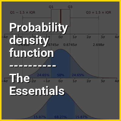
In descriptive statistics, the interquartile range (IQR) is a measure of statistical dispersion, which is the spread of the data. The IQR may also be called the midspread, middle 50%, fourth spread, or H‑spread. It is defined as the difference between the 75th and 25th percentiles of the data. To calculate the IQR, the data set is divided into quartiles, or four rank-ordered even parts via linear interpolation. These quartiles are denoted by Q₁ (also called the lower quartile), Q₂ (the median), and Q₃ (also called the upper quartile). The lower quartile corresponds with the 25th percentile and the upper quartile corresponds with the 75th percentile, so IQR = Q₃ −  Q_1.

The IQR is an example of a trimmed estimator, defined as the 25% trimmed range, which enhances the accuracy of dataset statistics by dropping lower contribution, outlying points. It is also used as a robust measure of scale It can be clearly visualized by the box on a box plot.

The Born rule is a postulate of quantum mechanics that gives the probability that a measurement of a quantum system will yield a given result. In one commonly used application, it states that the probability density for finding a particle at a given position is proportional to the square of the amplitude of the system's wavefunction at that position. It was formulated and published by German physicist Max Born in July 1926.

Given random variables ${\displaystyle X,Y,\ldots }$, that are defined on the same probability space, the multivariate or joint probability distribution for ${\displaystyle X,Y,\ldots }$ is a probability distribution that gives the probability that each of ${\displaystyle X,Y,\ldots }$ falls in any particular range or discrete set of values specified for that variable. In the case of only two random variables, this is called a bivariate distribution, but the concept generalizes to any number of random variables.

The joint probability distribution can be expressed in terms of a joint cumulative distribution function and either in terms of a joint probability density function (in the case of continuous variables) or joint probability mass function (in the case of discrete variables). These in turn can be used to find two other types of distributions: the marginal distribution giving the probabilities for any one of the variables with no reference to any specific ranges of values for the other variables, and the conditional probability distribution giving the probabilities for any subset of the variables conditional on particular values of the remaining variables.

In statistics, a location parameter of a probability distribution is a scalar- or vector-valued parameter ${\displaystyle x_{0}}$, which determines the "location" or shift of the distribution. In the literature of location parameter estimation, the probability distributions with such parameter are found to be formally defined in one of the following equivalent ways:

• either as having a probability density function or probability mass function ${\displaystyle f(x-x_{0})}$; or
• having a cumulative distribution function ${\displaystyle F(x-x_{0})}$; or
• being defined as resulting from the random variable transformation ${\displaystyle x_{0}+X}$, where ${\displaystyle X}$ is a random variable with a certain, possibly unknown, distribution. See also § Additive noise.

A direct example of a location parameter is the parameter ${\displaystyle \mu }$ of the normal distribution. To see this, note that the probability density function ${\displaystyle f(x|\mu ,\sigma )}$ of a normal distribution ${\displaystyle {\mathcal {N}}(\mu ,\sigma ^{2})}$ can have the parameter ${\displaystyle \mu }$ factored out and be written as: $${\displaystyle g(x'=x-\mu |\sigma )={\frac {1}{\sigma {\sqrt {2\pi }}}}\exp \left(-{\frac {1}{2}}\left({\frac {x'}{\sigma }}\right)^{2}\right)}$$thus fulfilling the first of the definitions given above.

The margin of error is a statistic expressing the amount of random sampling error in the results of a survey. The larger the margin of error, the less confidence one should have that a poll result would reflect the result of a simultaneous census of the entire population. The margin of error will be positive whenever a population is incompletely sampled and the outcome measure has positive variance, which is to say, whenever the measure varies.

The term margin of error is often used in non-survey contexts to indicate observational error in reporting measured quantities.

In statistics, probability density estimation or simply density estimation is the construction of an estimate, based on observed data, of an unobservable underlying probability density function. The unobservable density function is thought of as the density according to which a large population is distributed; the data are usually thought of as a random sample from that population.

A variety of approaches to density estimation are used, including Parzen windows and a range of data clustering techniques, including vector quantization. The most basic form of density estimation is a rescaled histogram.

In quantum mechanics, a probability amplitude is a complex number used for describing the behaviour of systems. The square of the modulus of this quantity at a point in space represents a probability density at that point.

Probability amplitudes provide a relationship between the quantum state vector of a system and the results of observations of that system, a link that was first proposed by Max Born, in 1926. Interpretation of values of a wave function as the probability amplitude is a pillar of the Copenhagen interpretation of quantum mechanics. In fact, the properties of the space of wave functions were being used to make physical predictions (such as emissions from atoms being at certain discrete energies) before any physical interpretation of a particular function was offered. Born was awarded half of the 1954 Nobel Prize in Physics for this understanding, and the probability thus calculated is sometimes called the "Born probability". These probabilistic concepts, namely the probability density and quantum measurements, were vigorously contested at the time by the original physicists working on the theory, such as Schrödinger and Einstein. It is the source of the mysterious consequences and philosophical difficulties in the interpretations of quantum mechanics—topics that continue to be debated even today.